Evidently

DVCLive 可用于跟踪 Evidently 的结果。接下来我们通过一个示例进行演示。

设置

$ pip install dvc dvclive evidently pandas

加载数据

从 UCI 仓库加载数据并保存到本地。为了演示目的，我们将这些数据视为实时模型的输入数据。在生产环境中使用时，您应确保能够访问您的预测日志。

$ wget https://archive.ics.uci.edu/static/public/275/bike+sharing+dataset.zip
$ unzip bike+sharing+dataset.zip

import pandas as pd

df = pd.read_csv("raw_data/day.csv", header=0, sep=',', parse_dates=['dteday'])
df.head()

这就是它的样子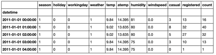： Sample data

定义列映射

您应指定分类特征和数值特征，以便 Evidently 对每种类型执行正确的统计检验。虽然 Evidently 可以自动解析数据结构，但手动指定列类型可以最大限度地减少错误。

from evidently.pipeline.column_mapping import ColumnMapping

data_columns = ColumnMapping()
data_columns.numerical_features = ['weathersit', 'temp', 'atemp', 'hum', 'windspeed']
data_columns.categorical_features = ['holiday', 'workingday']

定义要记录的内容

指定您希望计算的指标。在此案例中，您可以生成数据漂移报告，并记录每个特征的漂移分数。

from evidently.report import Report
from evidently.metric_preset import DataDriftPreset


def eval_drift(reference, production, column_mapping):
    data_drift_report = Report(metrics=[DataDriftPreset()])
    data_drift_report.run(
        reference_data=reference, current_data=production, column_mapping=column_mapping
    )
    report = data_drift_report.as_dict()

    drifts = []

    for feature in (
        column_mapping.numerical_features + column_mapping.categorical_features
    ):
        drifts.append(
            (
                feature,
                report["metrics"][1]["result"]["drift_by_columns"][feature][
                    "drift_score"
                ],
            )
        )

    return drifts

您可以通过从 Evidently 提供的预设（Preset）或指标（Metric）中选择不同的选项，来调整需要计算的内容。

定义比较窗口

指定作为参考的时间段：Evidently 将以此作为比较基准。然后，您应选择作为实验处理的时间段。这模拟了生产模型的运行过程。

#set reference dates
reference_dates = ('2011-01-01 00:00:00','2011-01-28 23:00:00')

#set experiment batches dates
experiment_batches = [
    ('2011-01-01 00:00:00','2011-01-29 23:00:00'),
    ('2011-01-29 00:00:00','2011-02-07 23:00:00'),
    ('2011-02-07 00:00:00','2011-02-14 23:00:00'),
    ('2011-02-15 00:00:00','2011-02-21 23:00:00'),
]

在 DVC 中运行并记录实验

有两种方式可以使用 DVCLive 跟踪 Evidently 的结果：

您可以将批次中每个项目的结果保存在一个单一实验中（每个实验对应一次 git 提交），分步骤保存
或者您可以将批次中每个项目的结果保存为独立的实验

我们将演示这两种方法，并向您展示如何在不依赖特定 IDE 的情况下检查结果。但是，如果您使用的是 VSCode，我们建议使用 VS Code 的 DVC 扩展来查看结果。

1. 单一实验

from dvclive import Live

with Live() as live:
    for date in experiment_batches:
        live.log_param("begin", date[0])
        live.log_param("end", date[1])

        metrics = eval_drift(
            df.loc[df.dteday.between(reference_dates[0], reference_dates[1])],
            df.loc[df.dteday.between(date[0], date[1])],
            column_mapping=data_columns,
        )

        for feature in metrics:
            live.log_metric(feature[0], round(feature[1], 3))

        live.next_step()

然后您可以使用以下方式检查结果：

$ dvc plots show

并检查生成的 dvc_plots/index.html，其外观应如下所示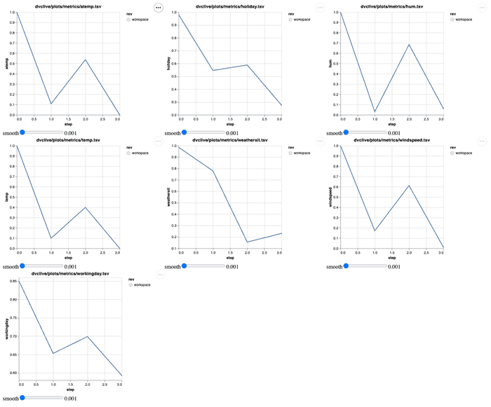： DVC plot show

在 Jupyter Notebook 环境中，只需使用 Live(report="notebook") 即可将图表作为单元格输出显示。

2. 多个实验

from dvclive import Live

for step, date in enumerate(experiment_batches):
    with Live() as live:
        live.log_param("begin", date[0])
        live.log_param("end", date[1])
        live.log_param("step", step)

        metrics = eval_drift(
            df.loc[df.dteday.between(reference_dates[0], reference_dates[1])],
            df.loc[df.dteday.between(date[0], date[1])],
            column_mapping=data_columns,
        )

        for feature in metrics:
            live.log_metric(feature[0], round(feature[1], 3))

您可以使用以下方式检查结果：

$ dvc exp show

────────────────────────────────────────────────────────────────────────────────────────────────────────────────────────────────────────────────────────────────
  Experiment                 Created    weathersit    temp   atemp     hum   windspeed   holiday   workingday   step   begin                 end
 ────────────────────────────────────────────────────────────────────────────────────────────────────────────────────────────────────────────────────────────────
  workspace                  -               0.231       0       0   0.062       0.012     0.275        0.593   3      2011-02-15 00:00:00   2011-02-21 23:00:00
  master                     10:02 AM            -       -       -       -           -         -            -   -      -                     -
  ├── a96b45c [muggy-rand]   10:02 AM        0.231       0       0   0.062       0.012     0.275        0.593   3      2011-02-15 00:00:00   2011-02-21 23:00:00
  ├── 78c6668 [pawky-arcs]   10:02 AM        0.155   0.399   0.537   0.684       0.611     0.588        0.699   2      2011-02-07 00:00:00   2011-02-14 23:00:00
  ├── c1dd720 [joint-wont]   10:02 AM        0.779   0.098   0.107    0.03       0.171     0.545        0.653   1      2011-01-29 00:00:00   2011-02-07 23:00:00
  └── d0ddb8d [osmic-impi]   10:02 AM        0.985       1       1       1           1      0.98        0.851   0      2011-01-01 00:00:00   2011-01-29 23:00:00
 ────────────────────────────────────────────────────────────────────────────────────────────────────────────────────────────────────────────────────────────────

在 Jupyter Notebook 环境中，您可以使用 Python DVC API 访问实验结果：

import dvc.api

dvc.api.exp_show()